Training a segmentation Model

In this tutorial, you will learn how to train a segmentation model in Arkindex.

This section is to be followed and carried out after creating the ground-truth annotations.

Generating an export of the project

Browse to the page of the Europeana | Pellet project. Instructions to start an SQLite export are detailed in our guide to export a project. Once started, read how to monitor the status of your export.

Wait for your export to be Done before going further in this tutorial.

Using an SQLite database speeds things up and avoids making too many requests to the API, especially for large datasets.

Create a model

The training will save the model’s files as a new version on Arkindex. In this section, we will create the model that will hold this new version.

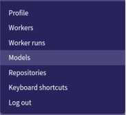
Click on Models in the top right dropdown (with your email address).

Figure 1. Browse to the Models page

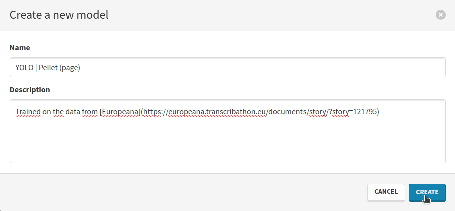
Click on the Create blue button to create a new model. This will open a modal where you can fill your model’s information. It is a good idea to name the model after:

the Machine Learning technology used,
the dataset,
the type of element present in the dataset.

In our case, we are training:

a YOLO26 model,
on the Pellet dataset,
on page elements.

A suitable name would be YOLO | Pellet (page). In the description, you can add a link towards the dataset on Europeana. The description supports Markdown input.

Figure 2. Create a new model

An Arkindex model object can hold multiple versions. If you do another training under different conditions (for a longer period of time, …), you do not have to create a brand new model again.

Start your training process

Now that you have a dataset and a model, we can create the training process.

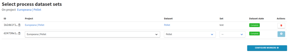
Create a process using all sets of the dataset.

Select the Pellet dataset and select All sets to add all three sets to the process.

Press the button in Actions column to confirm.

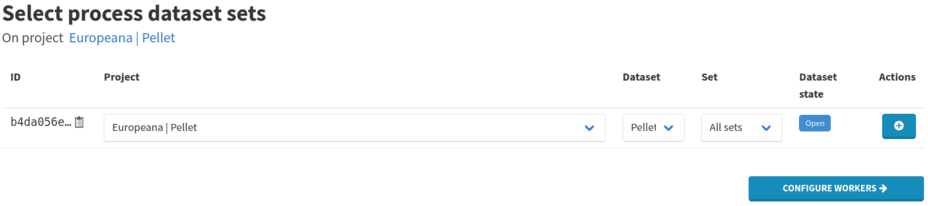
Figure 3. Select the dataset and its sets

Use the Configure workers button to move on to worker selection.

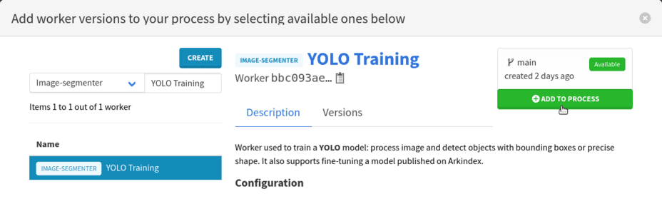
Proceed to workers configuration. Press the Select workers button, filter by the Object detector worker type, then search for YOLO Training and press the Enter keyboard key.

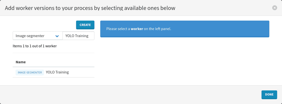
Figure 4. Search for the YOLO Training worker

Click on the name of the worker on the left.

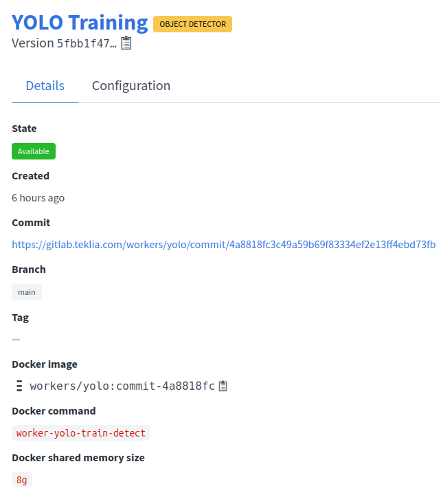
Learn more about the available worker version by clicking on the box with the details on the right.

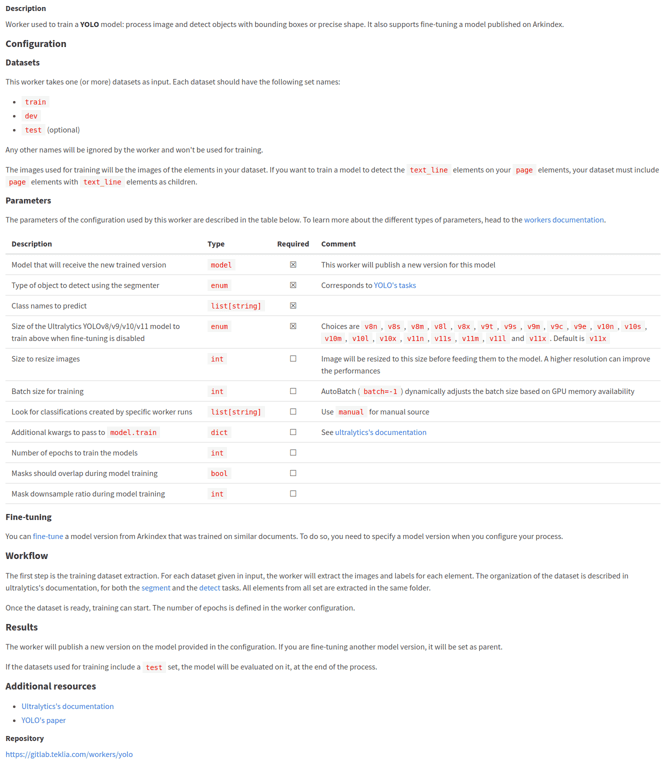
Access the details of the worker version

Figure 5. Click on the box with the worker version details.

This will open the page with the description of the worker and its configuration.

Check out the details of the worker version

Figure 6. The details of the worker version.

Check out the configuration of the worker version

Figure 7. The configuration of the worker version.

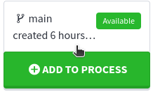
On the page with the process configuration, select the recommended version by clicking on the Add to process button in the top-right corner.

Figure 8. Add the YOLO Training worker to the process

Then you can close the modal by clicking on the Done button on the bottom right.

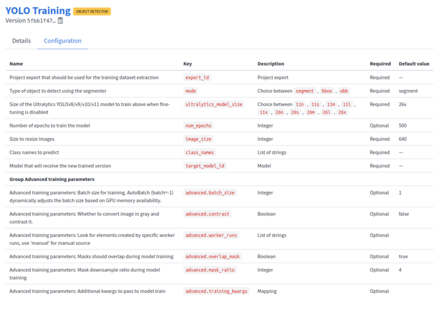
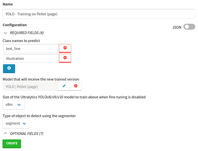
Configure the YOLO Training worker by clicking on the button in the Configuration column. This will open a new modal, where you can pass specific parameters used for training. The full description of the fields is available on the worker’s description page.

Figure 9. Worker’s description

Select New configuration on the left column, to create a new configuration. Again, name it after the dataset you are using.

Figure 10. Configure the worker

The most important parameters are:

Project export that should be used for the training dataset extraction: select the export that you just generated,
Type of object to detect using the segmenter:
- a segmenter will produce masks (polygons),
- a detector will produce bounding boxes (rectangles),
Size of the Ultralytics YOLOv8/v9/v10/v11 model to train above when fine-tuning is disabled: pick the medium version titled 26m here,
Number of epochs to train the model (optional): the default value is good enough but you can set it to a larger number if you want to train for a longer period of time.
Size to resize images: a higher value can improve the performances but will also increase the memory usage,
Class names to predict: add the slugs of the types that the model will predict, text_line and illustration,
Model that will receive the new trained version: search for the name of your model.

Click on Create then Select when you are done filling the fields. Your process is ready to go.

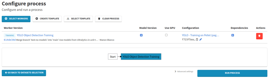
Figure 11. Configured process, ready to launch

Click on the Run process button to launch the process.

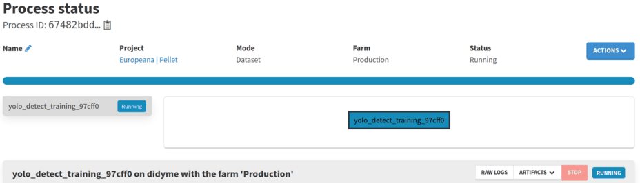
Figure 12. Training process is running

While it is running, the logs of the tasks are displayed. Multiple things happen during this process:

The dataset is converted into the right format for YOLO v8 segmentation models,
Training starts, for as long as needed,
Evaluation on all three splits,
The new model is published on Arkindex.

Evaluation

Training logs

Evaluation results are displayed at the end of the training logs.

Figure 13. The process logs

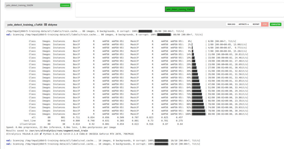
Note that YOLO uses the keyword val during the evaluation stage, even though it is run over the three splits (train, dev and test) sequentially.

To know which split is being evaluated, check the data used for the evaluation. For example, the first block (visible in the figure above) shows the performance over the train split as it loads data from /tmp/tmpa3j68dr5-training-data/all/labels/train.cache (note the train.cache at the end).

The first lines, with the progress bar, correspond to the part where the worker processed each image of the split. After that section, there is a table explaining the metrics on this split. The last line with the progress bar gives the header of the columns below.

the Class column explains which part of the images is evaluated
- all corresponds to the global performance of the model over all the examples,
- text_line line corresponds to the performance of the model regarding text_line segmentation,
- illustration line corresponds to the performance of the model regarding illustration segmentation.
the Images column gives the number of pages relevant for the line,
the Instances column gives the number of objects used to compute the metric,
the next four columns relate to the evaluation of objects of type "box" (rectangles). We are mostly interested in segmentation (polygons) so we can skip these.
the last four columns relate to the evaluation of objects of type "mask" (polygons). They correspond to the following metrics:
- P stands for Precision. It measures the accuracy of the detected objects, indicating how many detections were correct.
- R stands for Recall. It measures the ability to identify all instances of objects in the images.
- map50 stands for Mean Average Precision calculated at an intersection over union (IoU, i.e. overlap between predicted and actual boundary) threshold of 0.50. It measures the model’s accuracy considering only the "easy" detections.
- map50-95 stands for Mean Average Precision calculated at varying IoU thresholds, ranging from 0.50 to 0.95. It gives a comprehensive view of the model’s performance across different levels of detection difficulty.

We want to assess the model’s ability to generalize what it has learned to new examples. While the evaluation over the train and dev splits is relevant to make sure the model has actually learned something, only the test set contains images the model has never seen.

All metrics are important to evaluate the performance of the model. However, we generally want a high map50-95, as it provides a comprehensive evaluation of the model’s performance.

If you want more details, click the Artifacts button to list the artifacts and click results.tar.zst to download the training artifacts.

This type of archive is not natively supported by Windows. In that case, you will need an external archive manager tool like 7zip.

Figure 14. Download training artifacts

This archive has the following file structure:

one train folder: with graphs and sheets describing how the training went,
three eval_* folders: the evaluation results on all splits.

Make sure to take a look at these if you want to know more about your model’s performance.

Visit the page of your model to see your brand new trained model version. To do so, browse the Models page and search for your model.

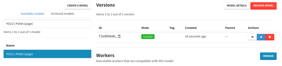
Figure 15. The new model version is displayed under the model details

You can download it to use it on your own or to process pages already on Arkindex, as described in the next section.

Evaluation by inference

Graphs are nice to get an idea of how the model performs on unknown data. However, it is easier to make yourself an idea when the predictions are actually displayed.

In this section, you will learn to process the test set of your dataset with your newly trained model.

Creating the process

Browse to the project you created in the earlier steps of the tutorial.

Click on Create training process in the Processes menu. Select your dataset but only keep the test set.

Figure 16. Create a process on the 'test' set

Click on Configure workers to move on to worker selection. Press the Select workers button, filter by the Image-segmenter worker type, search for YOLO Inference and press the Enter keyboard key. Just like we did in the previous sections, click on the name of the worker on the left and select the recommended version by clicking on the Add to process button in the top-right corner.

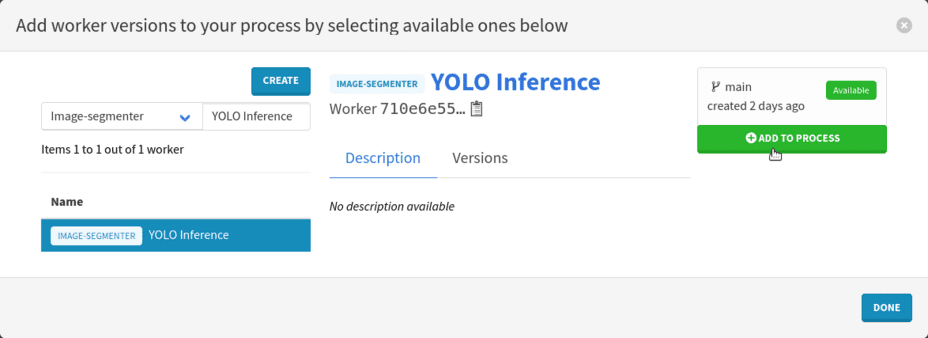
Figure 17. Add the YOLO Inference worker to the process

Close the modal by clicking on the Done button on the bottom right.

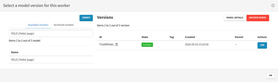
Now it is time to select the model you trained. Click on the button in the Model version column. In the modal that opens:

Look for the name of your trained model,
Add the model version by clicking on Use in the Actions column,
Close the modal by clicking on Ok, in the bottom right corner.

Figure 18. Add your trained model to the process

The process is ready and you can launch it using the Run process button. Wait for its completion before moving to the next step.

Visualizing predictions

To see the predictions of your model, browse back to the test folder in your project. There you can click on the first page displayed.

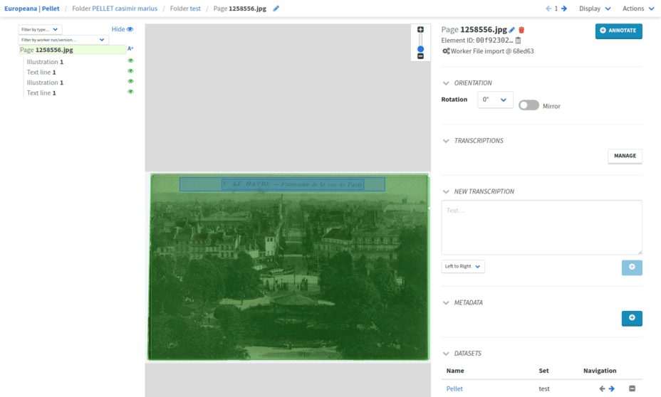
Figure 19. A page of the test set with annotations and predictions

On all pages of the test set, you can see both the annotations and the predictions. To know the difference between ground truth and predictions, look at the details of each element.

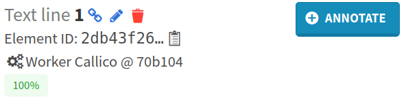
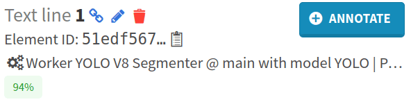
Figure 20. A text line annotated by a human

Figure 21. A text line predicted by the model

On the elements annotated by humans, Callico is mentioned. On the predicted elements, YOLO is mentioned. The confidence score of the YOLO prediction is also displayed.

In this tutorial, we do not calculate evaluation scores for this segmentation model as it would require you to run scoring tools using sophisticated procedures outside the Arkindex and Callico frameworks.

Next step

If the model’s initial results are close to the ground truth annotations, you could use it on all your pages through a dedicated process.